Posted on: 2025-11-06

I have recently read more about Monte Carlo simulation and the law of large numbers. I opted for Python and a framework called Optuna to try different hyperparameters. I never used Optuna, but I recall from my machine learning master's degree that it is ideal to optimize toward a maximum value, which in my case would be the most optimal portfolio value to start retiring with some flexibility in terms of yearly withdrawals. Optuna optimizes hyperparameters using a Gaussian process with Bayesian optimization, allowing multiple criteria. I want to optimize the overall success of my retirement over the next 40+ years.

Additionally, I want to start the simulation with the smallest amount possible to optimize an early retirement. The Monte Carlo simulation is based on two different possibilities that I am experimenting with. One is taking the last 150 years of S&P 500 random year performance and aligning them for 40 years (or another period). It continues until there is convergence. The simulation removes the withdrawal amount each year, adjusted for inflation, until the total of 40 years is completed. It does that until the standard error is under half a percent, and then tries another combination of random numbers. The second experiment is more sophisticated in terms of randomness. Historically, the S&P 500 has never had more than four consecutive negative years and never experienced a more than 50% sequential drop. While randomly assigning the performance of each year in the second experiment, if the 5th year is negative, it selects another random performance. The same happens if the accumulation of sequence years goes under 50%. In both cases, when the system determines a year, it removes it from the dataset to ensure uniqueness.

Monte Carlo

The simulation uses Monte Carlo to generate several random combinations of performance every year over a specified period. My computer has many cores, and to run the simulation in parallel, I rely on multiprocessing

  if n_workers is None:
      n_workers = max(1, cpu_count() - 1)  # leave one core for OS/other tasks

  if chunk_size is None:
      # choose chunk_size so each worker gets a few thousand sims
      # avoid too many small tasks; tune for your memory
      chunk_size = max(1_000, n_sims // (n_workers * 4))

  # Create the task list of (chunk_size, seed, return_trajectories)
  tasks = []
  remaining = n_sims
  seed_base = np.random.SeedSequence().entropy  # base entropy
  worker_seed = int(seed_base) & 0x7FFFFFFF
  i = 0
  while remaining > 0:
      c = min(chunk_size, remaining)
      tasks.append((c, worker_seed + i, return_trajectories))
      remaining -= c
      i += 1

  with Pool(
      processes=n_workers,
      initializer=_init_worker,
      initargs=(
          returns,
          n_years,
          initial_balance,
          withdrawal,
          withdrawal_negative_year,
          go_back_year,
          random_with_real_life_constraints,
      ),
  ) as pool:
      results = pool.map(_simulate_chunk, tasks)

The code determines the number of processor to use (worker) and separate the number of simulations (n_sims) each process will use. Then, a list of task get a seed to generate randomness differently. Using the trick with the bitwise ensures that it remains in a 32-bit and the +1 ensures each worker has a unique seed, avoiding two workers generating the same random index for selecting past returns.

The pool.map runs the simulation and returns the result in results in the same order as the task. While not very important in our case, it simplifies the debugging slightly.

The Pool runs with an initializer that is a function called once per worker. In our case, it sets up some global variables that are specific to each process (not shared across processes). It enables performance gains between multiple simulations in the process, avoiding the costly transfer of data by parameter. Thus, it is helpful for performance optimization. The initargs are passed by parameter and contain lightweight information that determines how to start the simulation.

Once the function completes all the simulations, it returns an object that contains the initial parameter, as well as the returns and, optionally, the balance of the portfolio every year. That is optional because it becomes large, but in some cases, it might be helpful for illustration purposes.

At this point, we can run without adjusting the hyperparameter automatically, but by guessing some scenario. For example, a simulation with these hyperparameters:

simulation_data = run_simulation_mp(
    return_trajectories=False,
    n_sims=100_000,
    initial_balance=4_500_000,
    withdrawal=110_000,
    withdrawal_negative_year=88_000,
    random_with_real_life_constraints=True,
)

Returns

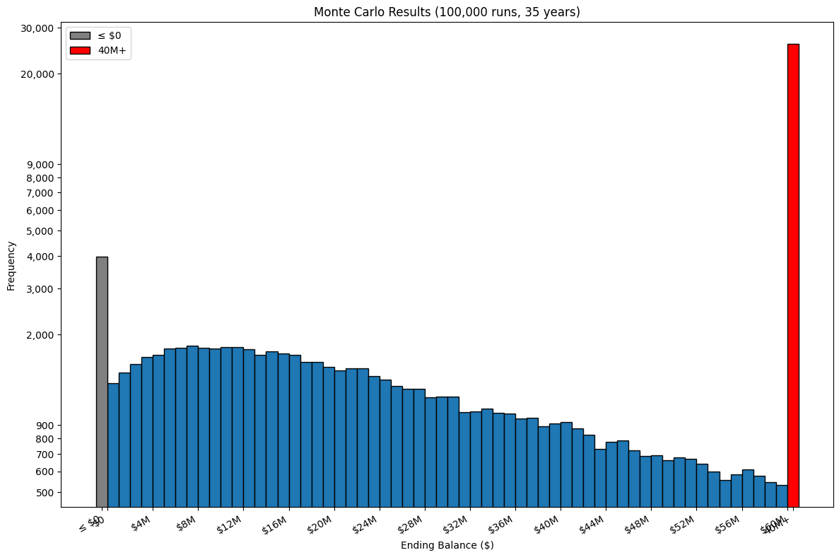
Simulation of 100,000 runs over 35 years took 2.53 seconds using constrained random.
The simulation starts using a portfolio balance of $4,500,000.

Probability portfolio survives 35 years: 96.0% if withdrawing $110,000 per year and in negative years $88,000 per year.
3,981 simulations ended ≤ $0.
96,019 simulations ended > $0.

Median ending balance: $29,593,789
10th, 25th, 75th, 90th percentile outcomes: ['$4,077,863', '$12,523,903', '$61,660,741', '$111,900,564']
Standard deviation of ending balances: $61,382,384
Mean ending balance: $48,546,195
Standard error: $194,108
Standard error / mean: $0.400%
95% confidence interval for the mean: $48,165,743 – $48,926,647

With this graph:

Another possibility is to show each of the simulation balances. With the same manual hyperparameters, the output is:

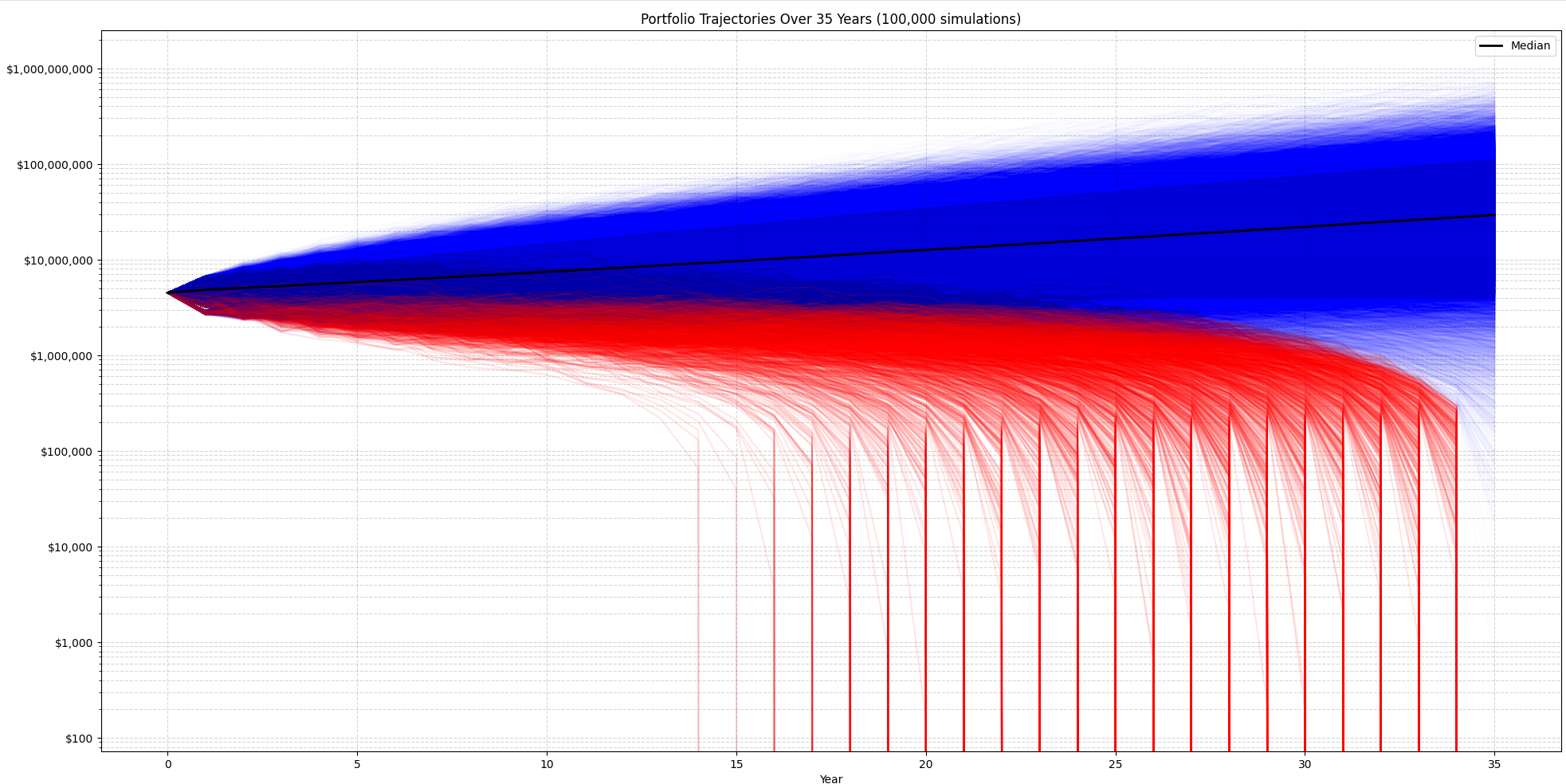
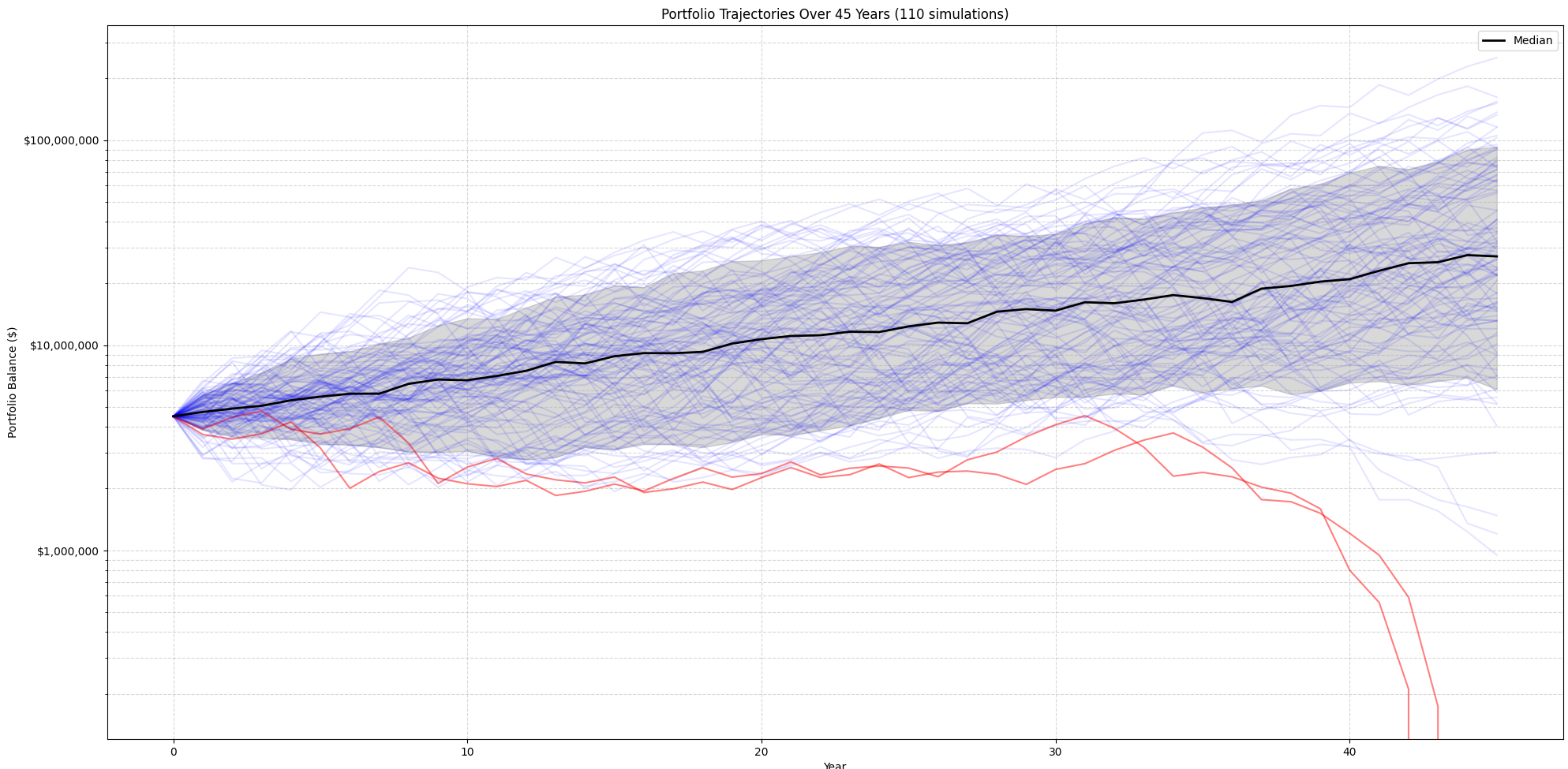
A third possibility is to simulate starting your retirement every year over the last 150 years and see how the portfolio would have performed. That illustrates the Great Recession, the crash of 2008, and similar events. It does not use Monte Carlo, but it's an interesting visualization to see how a portfolio would have worked in all these different past years. So, not random, more historically accurate.

Automatic Hyperparameters Optimization

Once the Monte Carlo is giving results that make sense from the input values, it is time to get the computer to try several combinations. The idea is to score each tentative to optimize toward a maximum value. The percentage of success is an important value, but ideally, we also want to be successful with the largest withdrawal and the lowest initial balance (retiring early). That part requires some experimentation, and I am still trying to determine the best scoring algorithm. Currently, I use the following scoring function:

gap_ratio = (withdrawal - withdrawal_negative_year) / withdrawal
gap_ratio = max(gap_ratio, 0)  # just in case
score = (
 threshold_power_map(prob_success, 0.85, 0.6) * 0.7
    + exponential(withdrawal, *WITHDRAWAL_RANGE, 2)
    * 0.05  # Encourage higher withdrawals
    + gap_ratio * 0.05  # encourage reducing withdrawals in bad years
    + inverse_exponential(initial_balance, *INITIAL_BALANCE_RANGE, 2)
    * 0.2  # Encourage lower initial balances
)

As you can see, 70% of the score is the probability of success, then 5% higher withdrawal from a range that I would be interested in withdrawing money every year. Then, 5% of the weight of the score is approximately how much money to withdraw when the year of the S&P 500 has a negative return. Finally, 20% of the initial balance, aiming for the lowest rate possible. I came up with an experiment. It was easy for the computer to find that a large initial balance is better, which was causing a bias toward late retirement. Similarly, initially, when focusing solely on the probability of succe

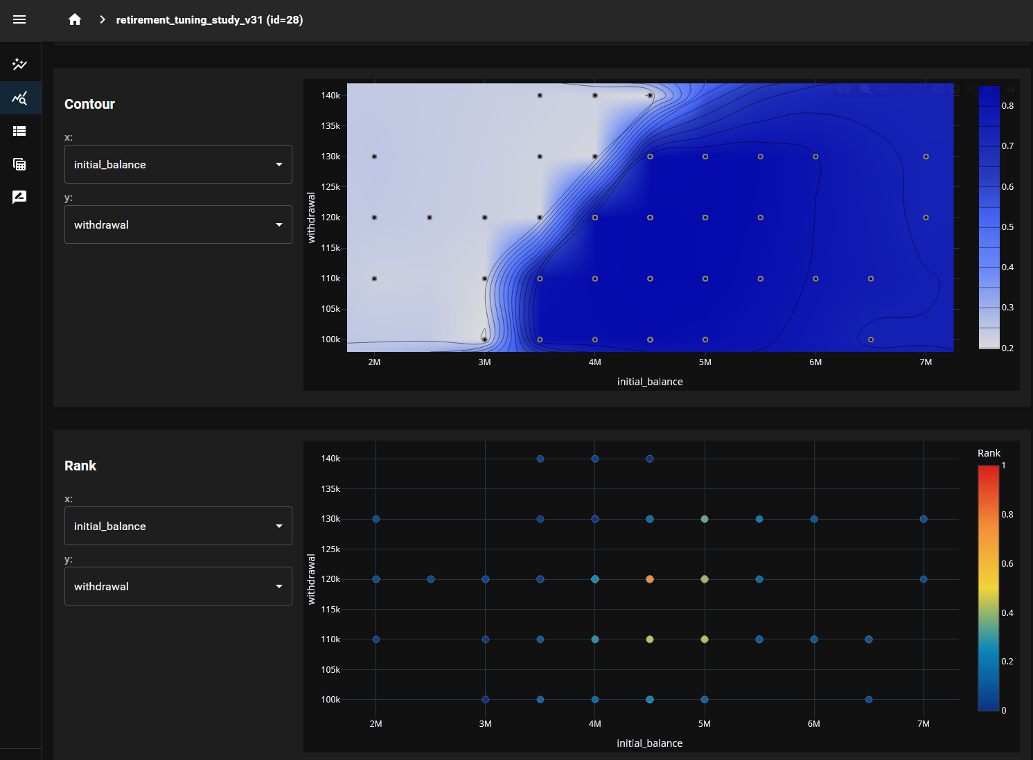
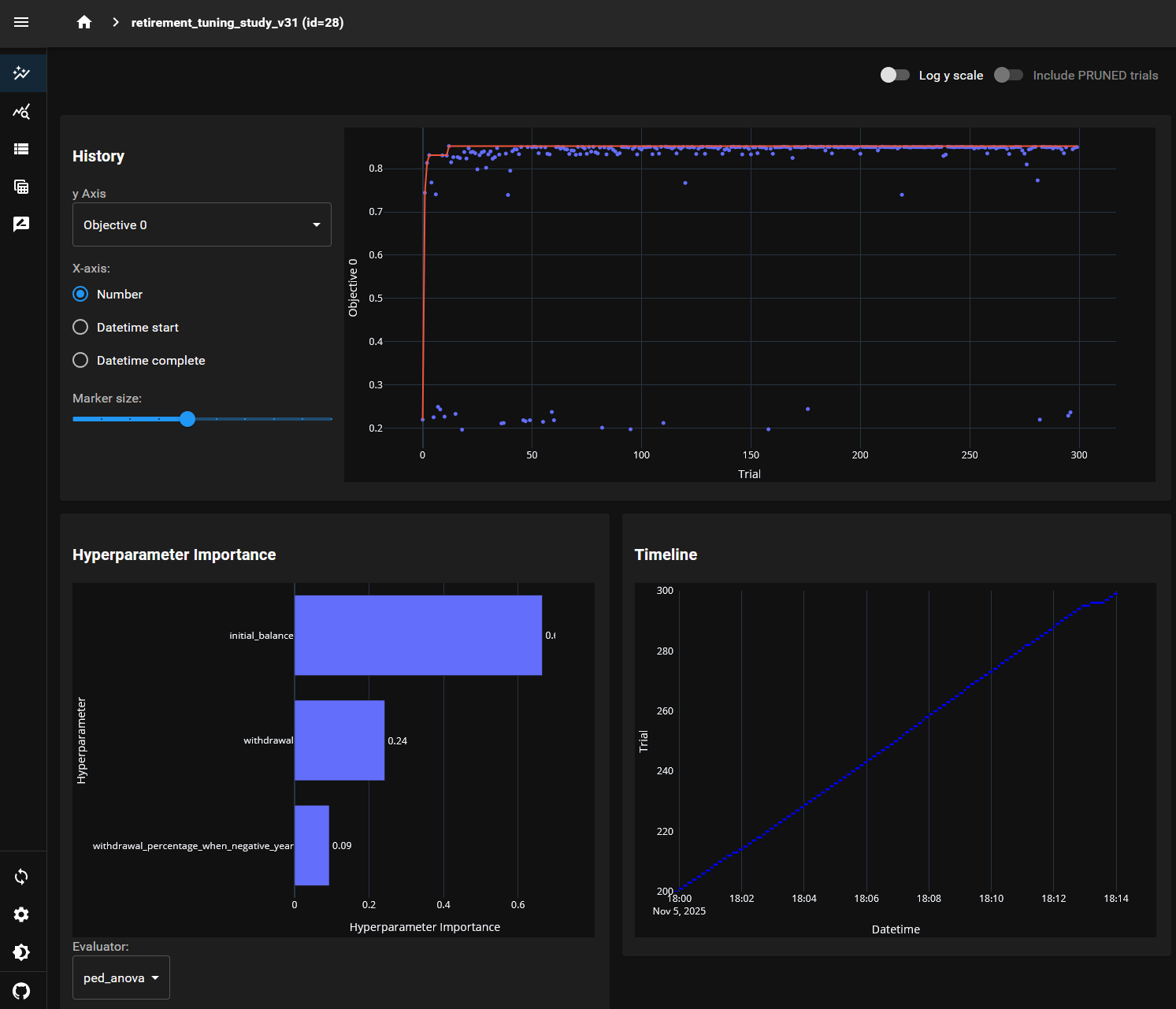
=== Optimization Results for retirement_tuning_study_v31 ===
Best Trial #12
  Initial Balance: $4,500,000.0
  Withdrawal: $110,000.0
  Withdrawal Negative Year: $88,000.0
  Withdrawal percentage: 0.8%
  Probability of Success: 94.13%
  Simulations Count used: 75,000
  Final Score: 85.1918%

And the web dashboard looks like:

Conclusion

The project of finding out the right balance of initial balance and withdrawal rate remains open. I am just getting started, and I will explore different hyperparameters and methods for calculating potential outcomes.